---
format: html
---

# A Poem (and a Painting) About the Suffering That Hides in Plain Sight

I’ve been reading this short, wry poem about suffering for more than 20 years.

How nice that it tells you in the first two words what it’s about.

No matter how familiar a poem is, rereading it always gives me a sense of first encounter, as though I’ve gone back to sleep and re-entered the dream through a different door.

About suffering they were never wrong,
The old Masters: how well they understood
Its human position: how it takes place
While someone else is eating or opening a window
    or just walking dully along;
---
format: closeread-html
---

# A Poem (and a Painting) About the Suffering That Hides in Plain Sight

I’ve been reading this short, wry poem about suffering for more than 20 years.

How nice that it tells you in the first two words what it’s about.

No matter how familiar a poem is, rereading it always gives me a sense of first encounter, as though I’ve gone back to sleep and re-entered the dream through a different door.

About suffering they were never wrong,
The old Masters: how well they understood
Its human position: how it takes place
While someone else is eating or opening a window
    or just walking dully along;
---
format:
  closeread-html:
    css: nytimes.css
---

# A Poem (and a Painting) About the Suffering That Hides in Plain Sight

I’ve been reading this short, wry poem about suffering for more than 20 years.

How nice that it tells you in the first two words what it’s about.

No matter how familiar a poem is, rereading it always gives me a sense of first encounter, as though I’ve gone back to sleep and re-entered the dream through a different door.

About suffering they were never wrong,
The old Masters: how well they understood
Its human position: how it takes place
While someone else is eating or opening a window
or just walking dully along; 
---
format:
  closeread-html:
    css: nytimes.css
---

# A Poem (and a Painting) About the Suffering That Hides in Plain Sight

I’ve been reading this short, wry poem about suffering for more than 20 years.

How nice that it tells you in the first two words what it’s about.

No matter how familiar a poem is, rereading it always gives me a sense of first encounter, as though I’ve gone back to sleep and re-entered the dream through a different door.

| About suffering they were never wrong,
| The old Masters: how well they understood
| Its human position: how it takes place
| While someone else is eating or opening a window
|     or just walking dully along;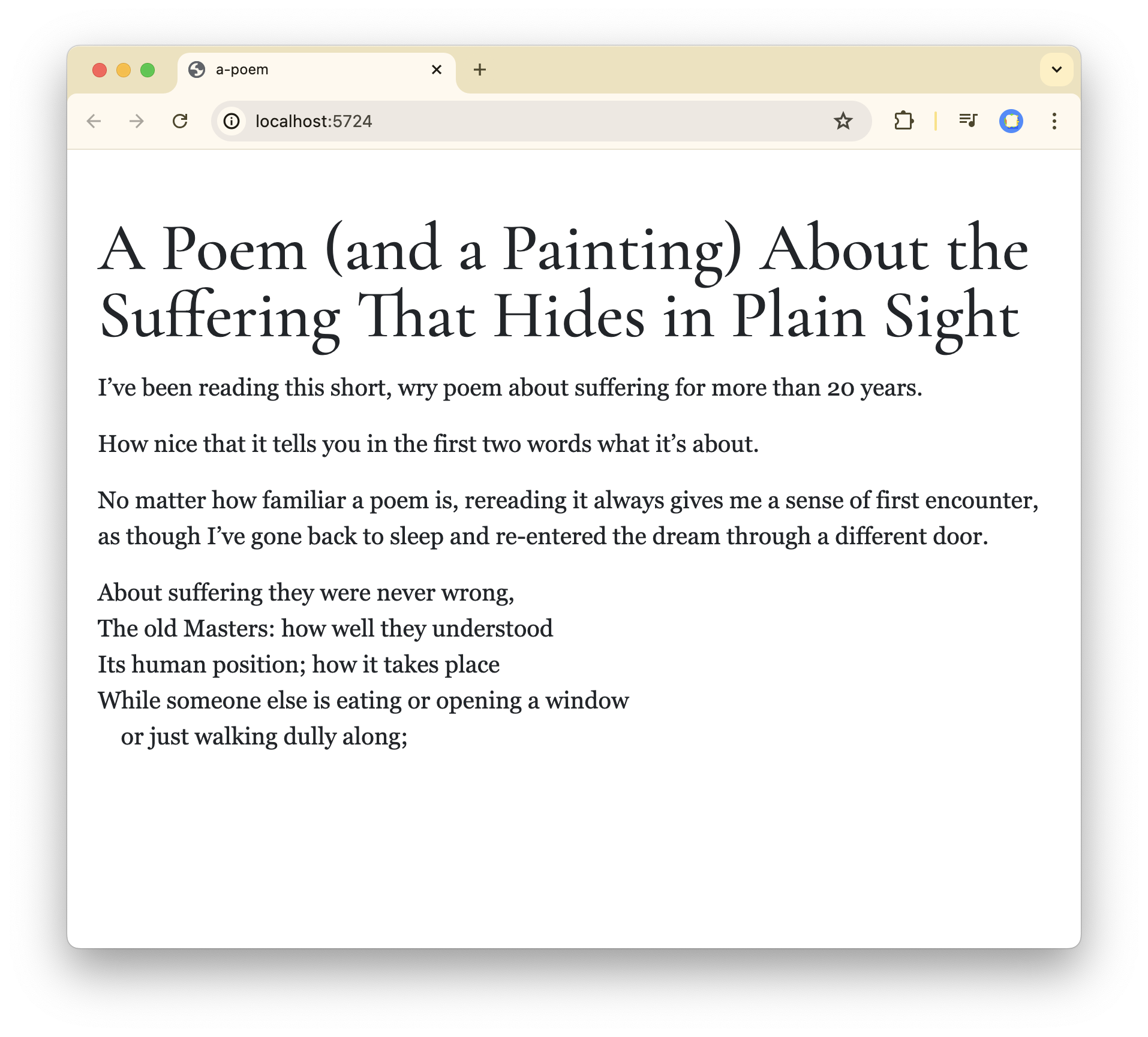
---
format:
closeread-html:
css: nytimes.css
---
:::{.cr-section}
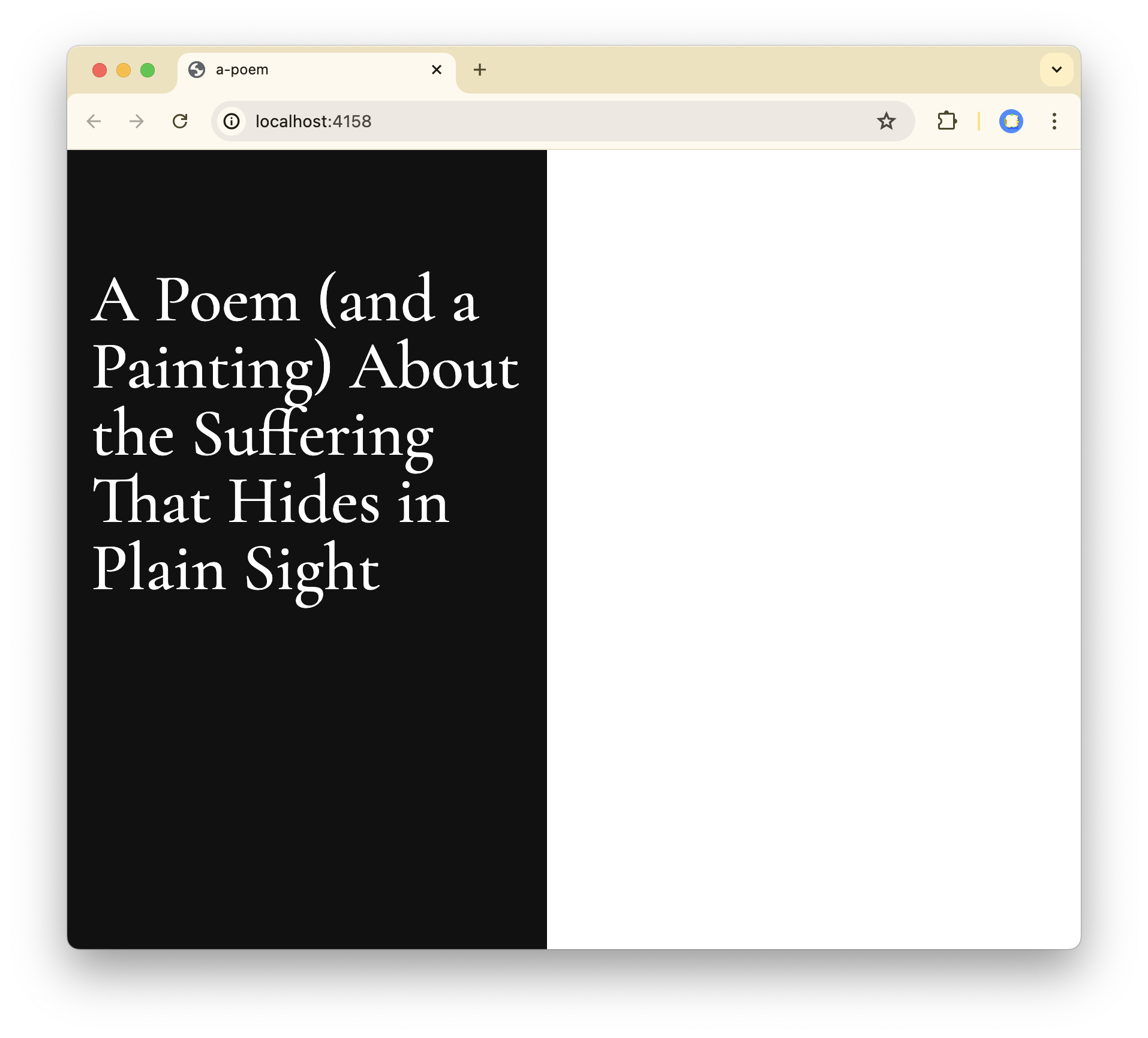
# A Poem (and a Painting) About the Suffering That Hides in Plain Sight
I’ve been reading this short, wry poem about suffering for more than 20 years.
How nice that it tells you in the first two words what it’s about.
No matter how familiar a poem is, rereading it always gives me a sense of first encounter, as though I’ve gone back to sleep and re-entered the dream through a different door.
| About suffering they were never wrong,
| The old Masters: how well they understood
| Its human position; how it takes place
| While someone else is eating or opening a window
| or just walking dully along;
::: 
---
format:
closeread-html:
css: cr-tufte.css
---
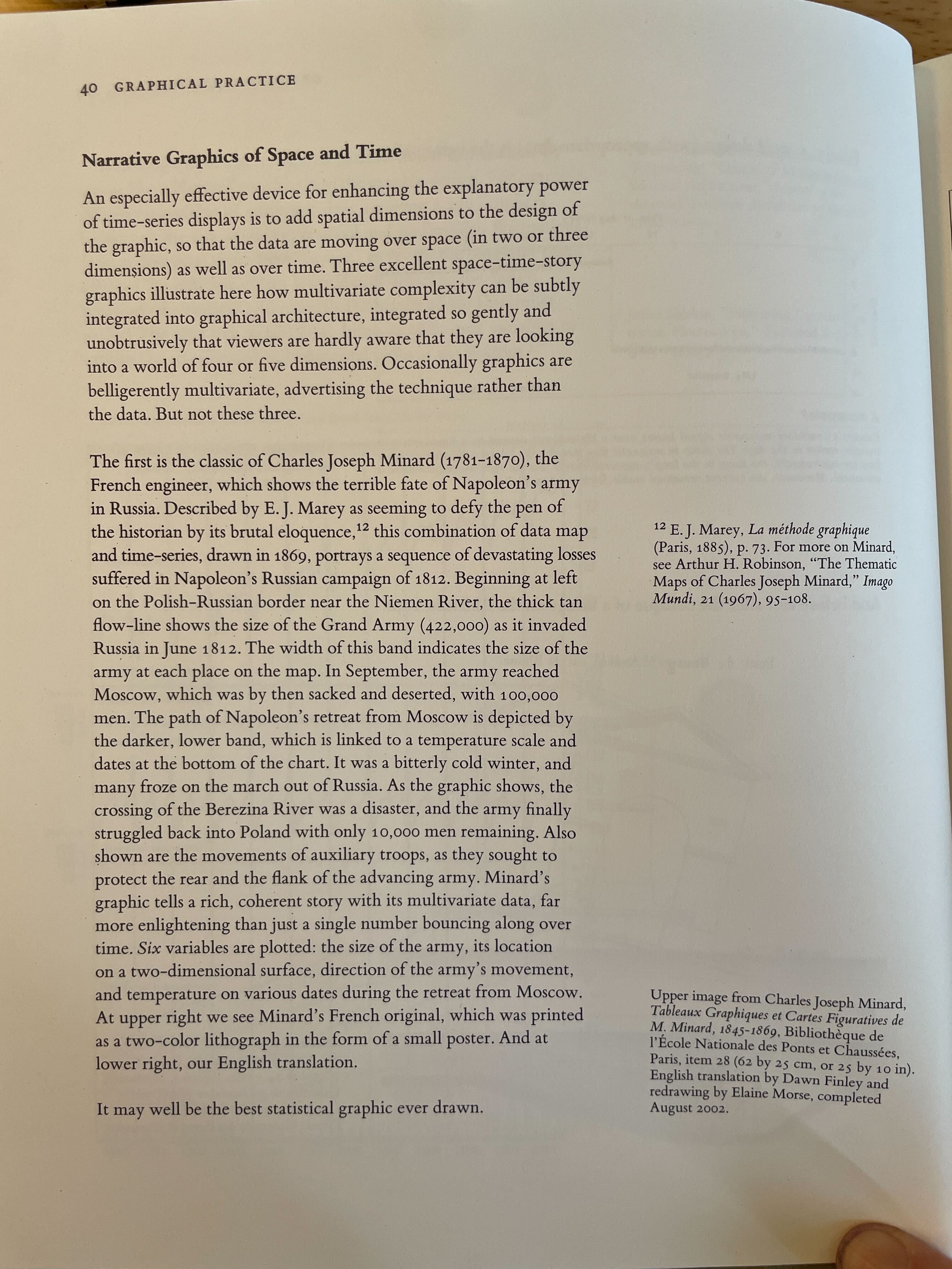
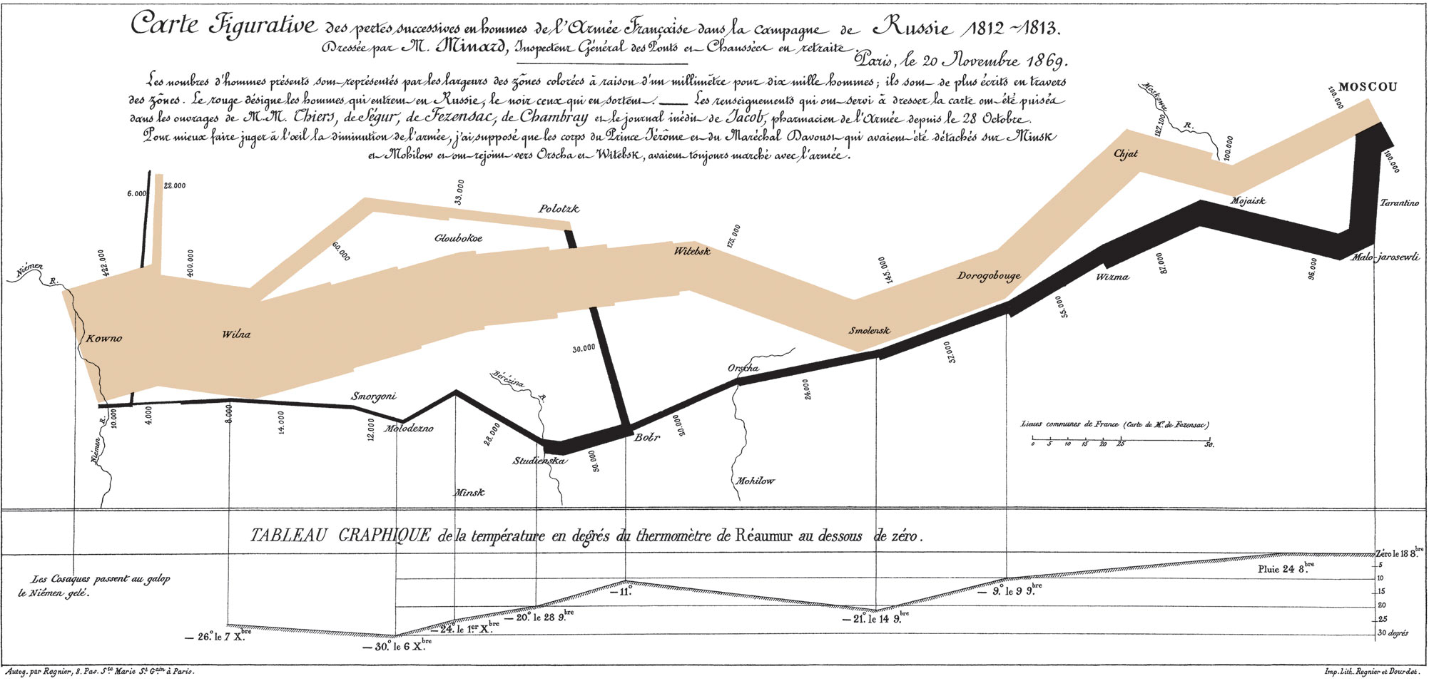
The first is the classic of Charles Joseph Minard (1781-1870), the French engineer, which shows the terrible fate of Napoleon's army in Russia. Described by E. J. Marey as seeming to defy the pen of the historian by its brutal eloquence, 12 this combination of data map and time-series, drawn in 1869, portrays a sequence of devastating losses suffered in Napoleon's Russian campaign of 1812.

Beginning at left on the Polish-Russian border near the Niemen River, the thick tan flow-line shows the size of the Grand Army (422,000) as it invaded Russia in June 1812.
The width of this band indicates the size of the army at each place on the map.
In September, the army reached Moscow, which was by then sacked and deserted, with 100,000 men.
The path of Napoleon's retreat from Moscow is depicted by the darker, lower band, which is linked to a temperature scale and dates at the bottom of the chart. It was a bitterly cold winter, and many froze on the march out of Russia.
As the graphic shows, the crossing of the Berezina River was a disaster, and the army finally struggled back into Poland with only 10,000 men remaining.
Also shown are the movements of auxiliary troops, as they sought to protect the rear and the flank of the advancing army.
Minard's graphic tells a rich, coherent story with its multivariate data, far more enlightening than just a single number bouncing along over time. Six variables are plotted: the size of the army, its location on a two-dimensional surface, direction of the army's movement, and temperature on various dates during the retreat from Moscow.
It may well be the best statistical graphic ever drawn.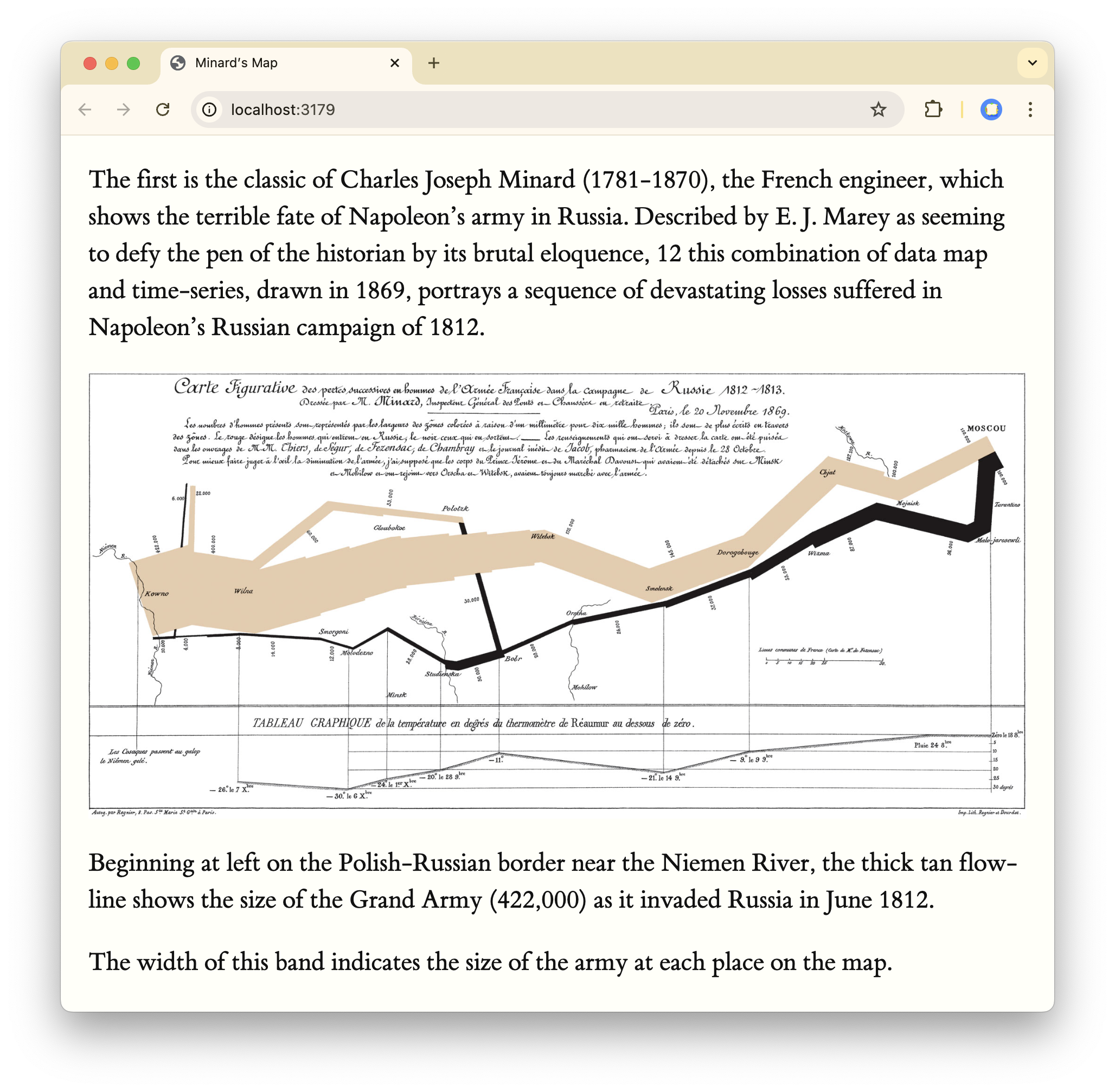
---
format: closeread-html
---
:::{.cr-section}
:::{focus-on="cr-dplyr"}
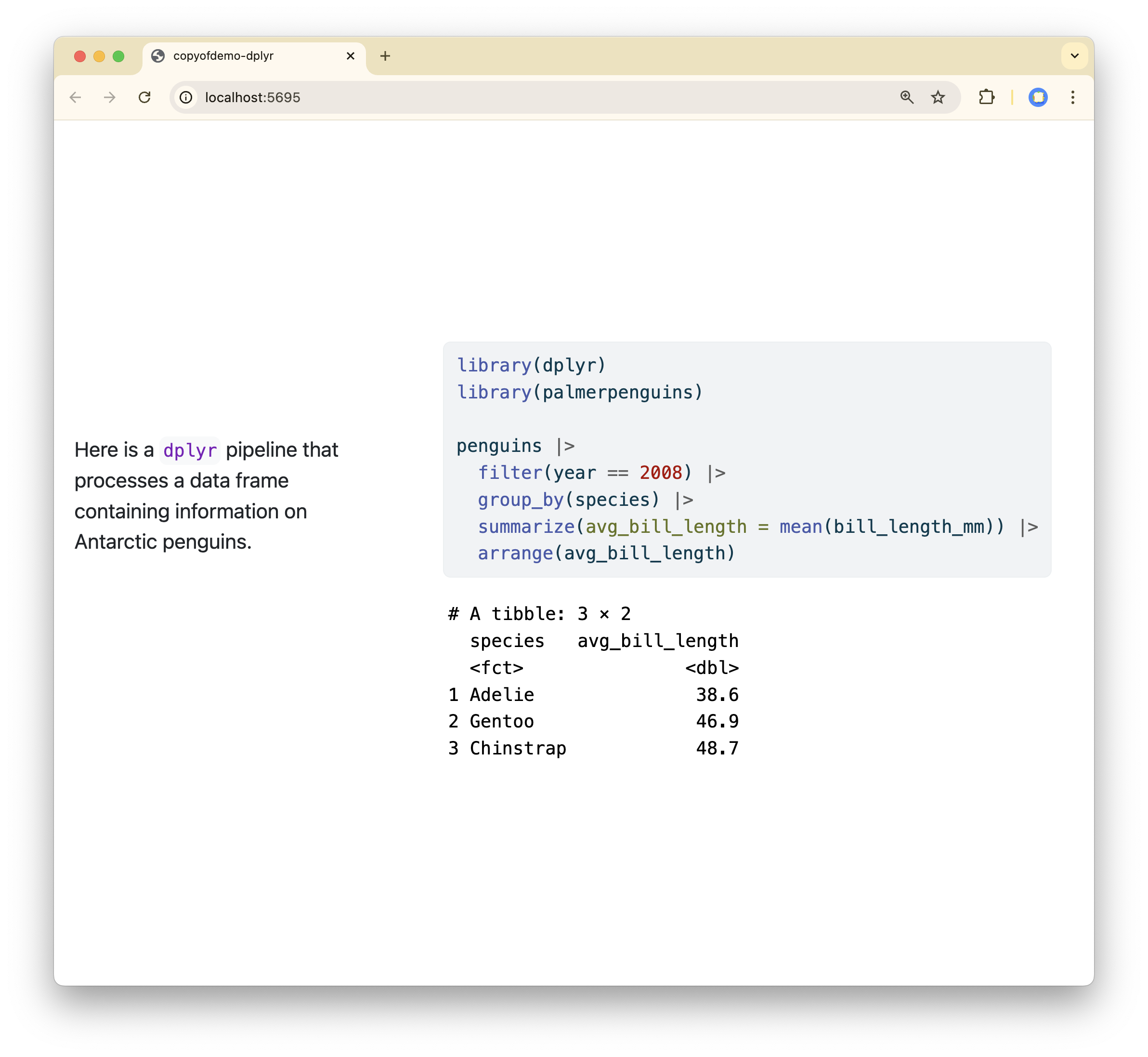
Here is a `dplyr` pipeline that processes a data frame containing information on Antarctic penguins.
:::
In the first two lines we load the `dplyr` package and the `palmerpenguins` package, which contains the data frame.
The main block of code is referred as a pipeline or chain. Each line starts with a function and ends with a pipe, `|>`.
:::{#cr-dplyr}
```{r}
#| echo: true
#| message: false
library(dplyr)
library(palmerpenguins)
penguins |>
filter(year == 2008) |>
group_by(species) |>
summarize(avg_bill_length = mean(bill_length_mm)) |>
arrange(avg_bill_length)
```
:::
:::
---
format: closeread-html
---
::::{.cr-section layout="overlay-center"}
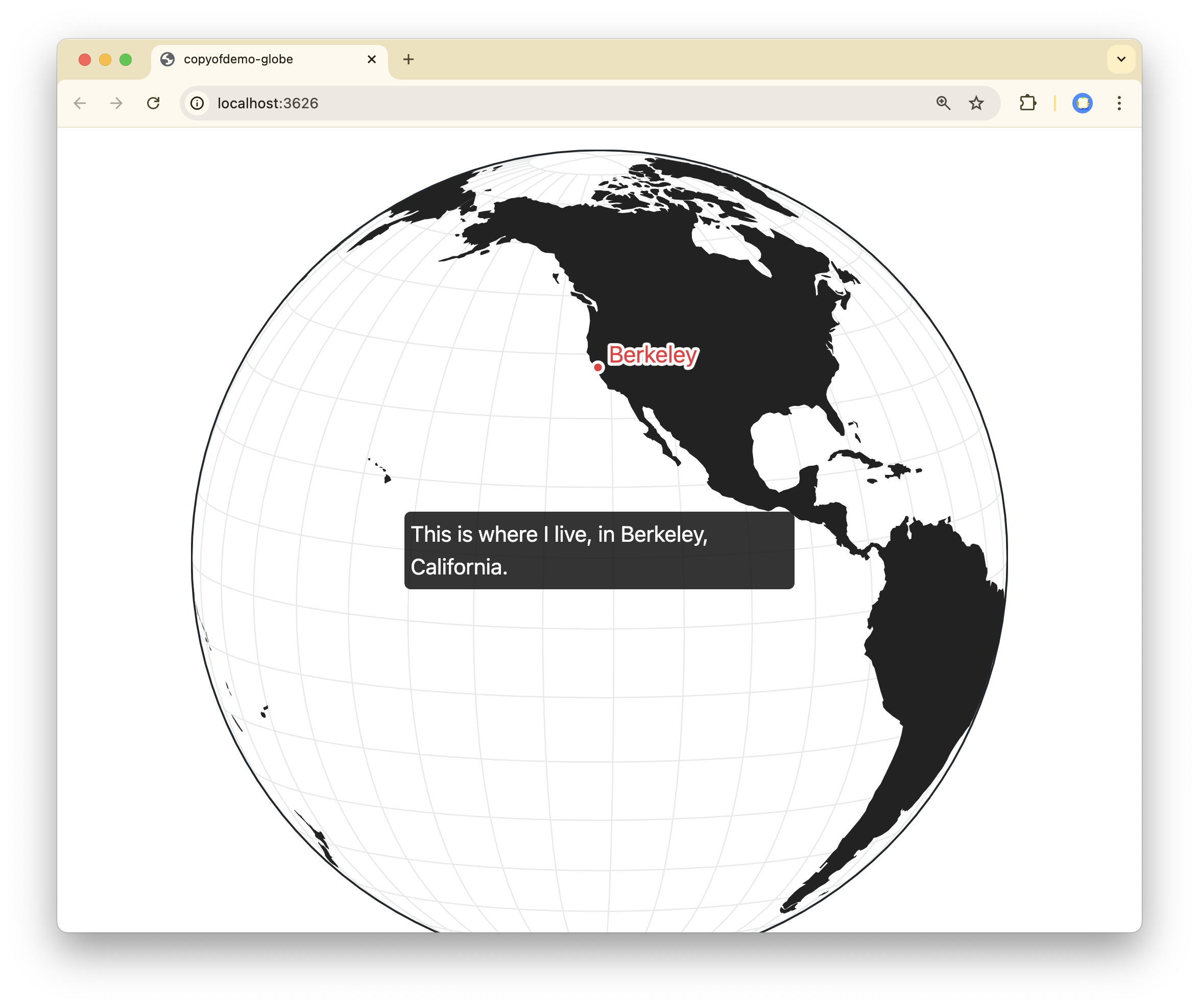
This is where I live, in Berkeley, California. @cr-globe
My collaborator James lives very, very, far away.
:::{#cr-globe}
```{ojs}
world = FileAttachment("naturalearth-land-110m.geojson").json()
cities = [{ name: "Berkeley", lat: 37.8715, lon: -122.2730 },
{ name: "Melbourne", lat: -37.8136, lon: 144.9631 }]
```
```{ojs}
Plot.plot({
marks: [
Plot.graticule(),
Plot.geo(world, {
fill: "#222222"
}),
Plot.sphere(),
Plot.dot(cities, {
x: "lon",
y: "lat",
fill: "#eb343d",
stroke: "white",
strokeWidth: 5,
paintOrder: "stroke",
size: 6
}),
Plot.text(cities, {
x: d => d.lon + 2,
y: d => d.lat + 2,
text: "name",
fill: "#eb343d",
stroke: "white",
strokeWidth: 5,
paintOrder: "stroke",
fontSize: 18,
textAnchor: "start"
}),
],
projection: {
type: "orthographic",
rotate: [122, -10]
}
})
```
:::
::::